Estimators
Question
Let $a_1, …, a_n \in \bR$ and let $\bar{a}$ be the average of ${a_1, …, a_n}$, i.e. $\bar{a} = \frac{1}{n} \sum_i a_i$. Which of the following statements is true:
- $\bar{a} = \argmin_{a’\in \bR} \sum_i a_i - a’$
- $\bar{a} = \argmin_{a’\in \bR} \sum_i (a_i - a’)^2$
Summarizing a (probability) distribution
We often want to summarize a distribution with one number. For example, the grades of a student, the incomes of citizen in a country, our beliefs about a certain unknown parameter. In statistics, this number is called an estimator. In this post we discuss some considerations for choosing an estimator.
Different objectives
One possible objective for an estimator $a^*$ is to minimize the expected distance from a sample from the distribution.
\[a^*_{(1)} = \argmin_{a'\in \bR} \int |x - a'| p(x) dx\]It turns out that this objective leads to $a^*_{(1)}$ such that
\[\int_{-\infty}^{a^*_{(1)}} p(x) dx = \int^{\infty}_{a^*_{(1)}} p(x) dx,\]which is the median.
Another objective is the following:
\[a^*_{(1)} = \argmin_{a'\in \bR} \int (x - a')^2 p(x) dx,\]which leads to the average, or expected value, of the distribution. I.e.
\[a^*_{(2)} = \bE_{p(x)}(x) = \int x p(x) dx.\]The last objective we discuss is the following:
\[a^*_{(3)} = \argmax_{a'\in \bR} p(a').\]Which is called the mode. In the context of parameter estimation, where the distribution is a posterior distribution, this estimator is called the maximum a posteriori probability (MAP) estimator. Closely related to this is the estimator
\[\theta_{\textrm{MLE}} = \argmax_{\theta' \in \bR} p(D|\theta),\]where \(p(D|\theta)\) is the likelihood of the data $D$ given a parameter $\theta$. Note that $p(D|\theta)$ as a function of $\theta$ is not a distribution.
Estimators in practice
1 urn
Consider an urn with $N$ balls of which $R$ are red. We draw $n$ balls from the urn without replacement of which $r$ are red. In the post Laplace’s Rule of Succession we saw that the posterior belief of the total number of red balls $R$ given total number of balls $N$, data $D = (n,r)$, and initial information about the setup of the experiment $I$ is given by
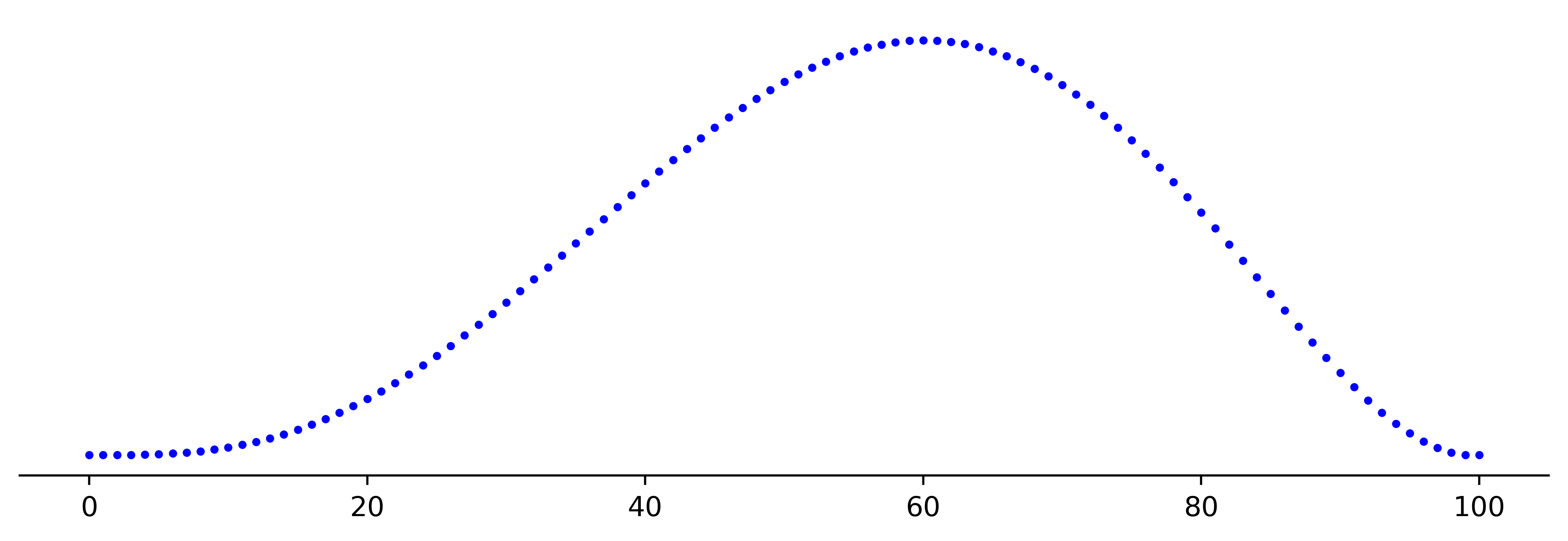
\[\begin{align*} p(R \mid DNI) = \binom{N+1}{n+1}^{-1} \binom{R}{r}\binom{N-R}{n-r}. \end{align*}\]Suppose $N=100, n=5, r=2$. The plot for the posterior looks as follows:

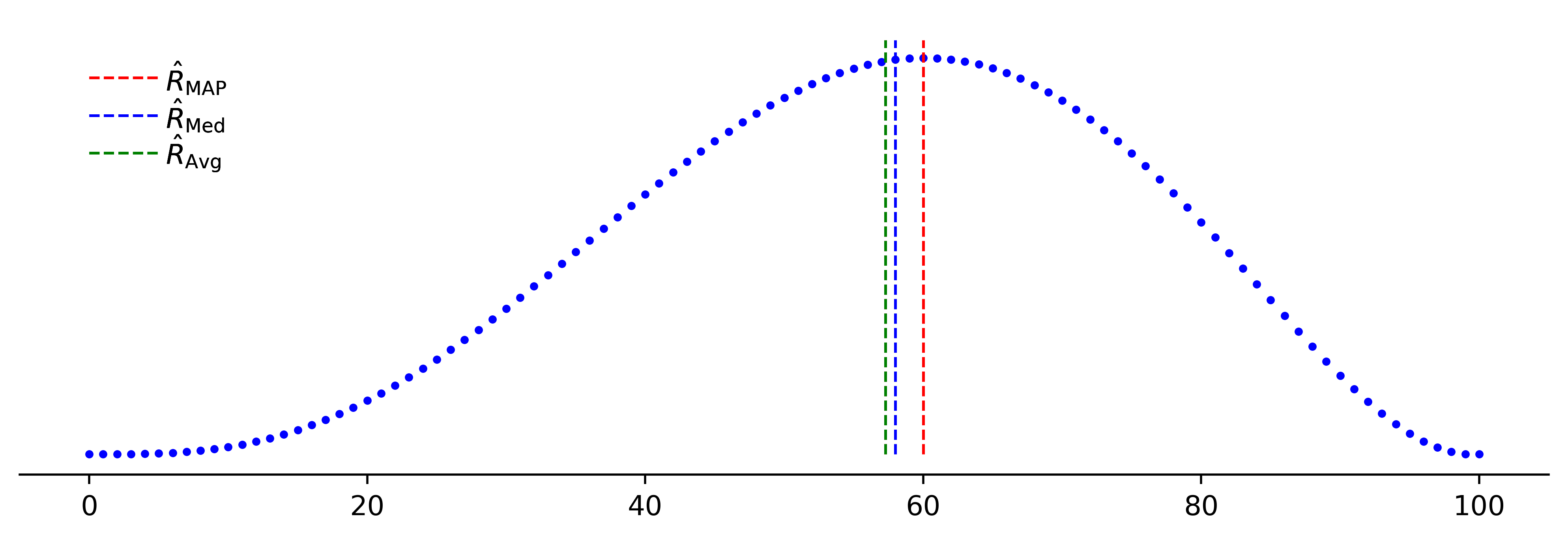
The estimators defined above can be plotted as follows:

Coin flip
Suppose we have a coin that comes up heads a fraction $\theta$. Assuming a uniform prior, the posterior belief about $\theta$ after having observed $r$ times heads after $n$ tosses is given by (see Appendix Laplace’s Rule of Succession):
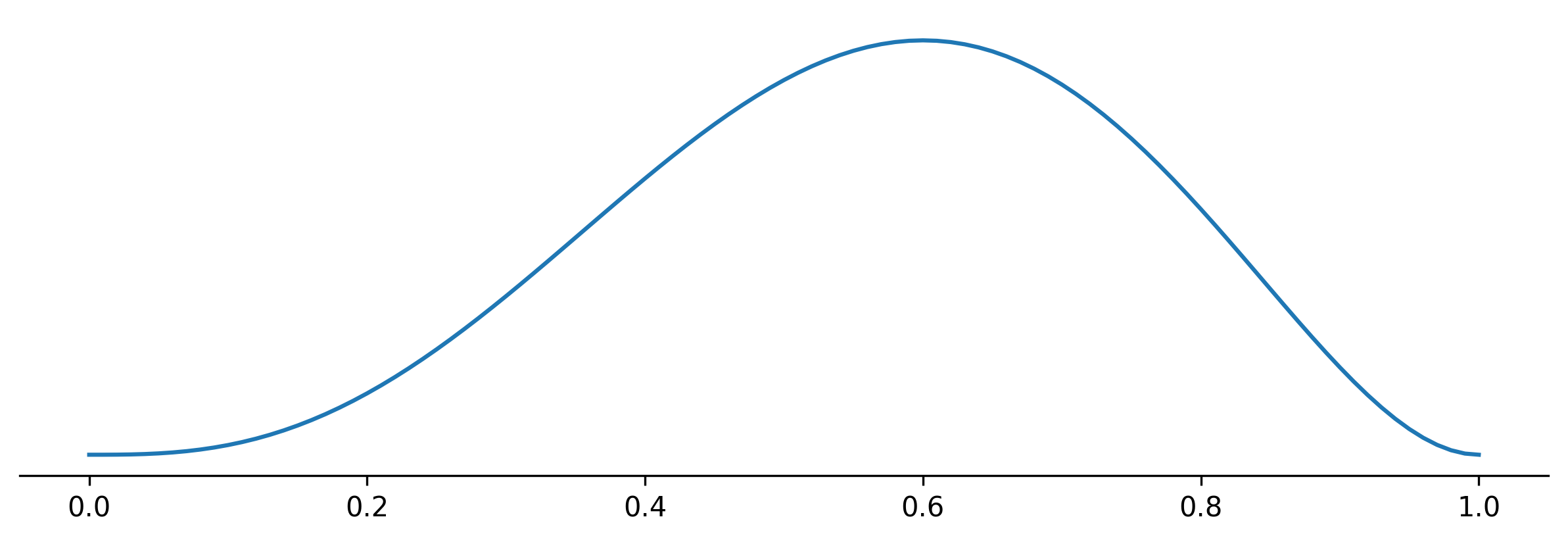
\[p(\theta|DI) = \frac{(n+1)!}{r!(n-r)!} \theta^r (1-\theta)^{n-r}.\]For $n = 5$ and $r=3$ the posterior plot looks as follows:

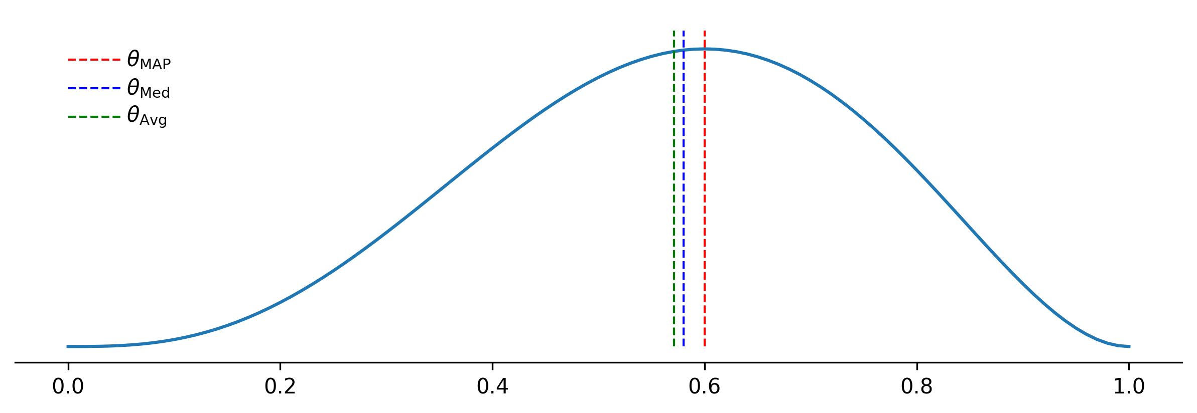
The estimators defined above can be plotted as follows:

Discussion
In different contexts different estimators are preferred. If you are gambling and $X$ is the random variable representing the profit (revenue - costs) of a bet, the estimator most of interest to you is the expectation of $X$.
If you have to represent the income distribution in a country, it could be argued that the median is the most representative estimator.
For (categorical) distribution without a clear distance measure on the sample space, the only possible estimator is the mode.
Summarizing the posterior of the coin flip
It could be argued that the value that summarizes the best the posterior \(p(\theta|DI)\) is the probability of thowing heads on the next throw, \(P(H_{n+1}|DI).\)
In we saw that this is given by
\[\begin{align*} P(H_{n+1}|DI) &= \int_0^1 P(H_{n+1}|\theta DI) p(\theta|DI) d \theta \\ &= \int_0^1 \theta p(\theta|DI) d \theta, \end{align*}\]which is the expected value of the posterior.